Tutorial - Memprot.GPCR-ModSim

Remco L. van den Broek, Rebecca V. Küpper, Xabier Bello, and Hugo Gutiérrez-de-Terán

Latest change: January 30th, 2024

[Download as PDF]

Overview

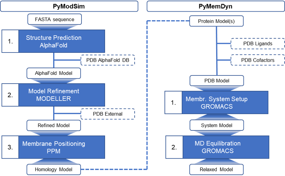
Memprot.GPCR-ModSim is an extension of the GPCR-ModSim web server, originally designed for the modeling and molecular dynamics (MD) equilibration of G-protein-coupled receptors (GPCRs). In the current version, the web server allows modeling and equilibration of ANY membrane protein. Homology models are gathered from AlphaFold-DB or predicted using the AlphaFold 2.0 engine for modeling protein sequences not stored within the database. MD equilibration is performed using refurbished pipelines designed for membrane embedding and solvation and performing MD simulations on the generated (or existing) membrane-protein models. The user can start a new project just from a FASTA sequence/UniProt ID, as well as uploading a pre-generated 3D structure (either experimental or modeled by any means), which importantly can include non-protein elements, such as ligand(s), structural waters, and ions. The flowchart of the server is depicted in Figure 1.

Tutorial

In this tutorial, we provide a step-by-step guide on operating the Memprot.GPCR-ModSim webserver. The following sections are found within this tutorial:

Homology modeling from a mutated sequence
Molecular Dynamics from a PDB file
Additional notes on ligands and cofactors

Homology modeling from a natural sequence

In this tutorial, we will show you how to follow a step-by-step recipe to create homology models of canonical membrane proteins (for mutated proteins see Homology modeling from mutated sequence). Here we demonstrate the process using the Histamine H3 receptor (HRH3) (UniProt ID: Q9Y5N1). To start our Histamine H3 project, we can either go to the ‘Projects’ tab > ‘Add a new sequence’, or directly go to ‘Model a GPCR’. Here, we will give the project the name Tutorial_HRH3.

Our first step is to specify the protein sequence. For proteins present in UniProt we can fill in the UniProt ID as follows (if needed, using the “Help” option within the sequence input will allow us to navigate through the Uniprot database in a new frame):

Q9Y5N1

Alternatively, we can specify the full sequence in FASTA format:

>sp|Q9Y5N1|HRH3_HUMAN Histamine H3 receptor OS=Homo sapiens OX=9606 GN=HRH3 PE=1 SV=2
MERAPPDGPLNASGALAGEAAAAGGARGFSAAWTAVLAALMALLIVATVLGNALVMLAFV
ADSSLRTQNNFFLLNLAISDFLVGAFCIPLYVPYVLTGRWTFGRGLCKLWLVVDYLLCTS
SAFNIVLISYDRFLSVTRAVSYRAQQGDTRRAVRKMLLVWVLAFLLYGPAILSWEYLSGG
SSIPEGHCYAEFFYNWYFLITASTLEFFTPFLSVTFFNLSIYLNIQRRTRLRLDGAREAA
GPEPPPEAQPSPPPPPGCWGCWQKGHGEAMPLHRYGVGEAAVGAEAGEATLGGGGGGGSV
ASPTSSSGSSSRGTERPRSLKRGSKPSASSASLEKRMKMVSQSFTQRFRLSRDRKVAKSL
AVIVSIFGLCWAPYTLLMIIRAACHGHCVPDYWYETSFWLLWANSAVNPVLYPLCHHSFR
RAFTKLLCPQKLKIQPHSSLEHCWK
 

We then press ‘Submit’ where we can check if the sequence is correctly read or imported from UniProt. With ‘Edit’, we can make any alterations to the sequence. If the sequence is correct, we press ‘Alpha Fold’ > ‘Submit’ to start the 3D structure protein modeling pipeline.

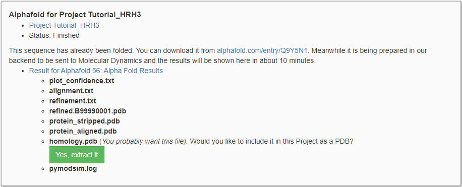
First, the modeling pipeline searches the AlphaFold-DB for existing models with identical sequences. Most proteins with a UniProt ID have a corresponding AlphaFold-DB structure. In our case, a matching structure has been found, and the structural model is retrieved from the database. Subsequently, the AlphaFold-DB structure is prepared for MD simulation (i.e. uncertain termini are cut, and uncertain loops are replaced with shorter poly-alanine chains). This process takes around 10 minutes, after which the results are provided as shown in Figure 2. Model_output.tgz contains the output of the preparation pipeline and can be downloaded and investigated by clicking on ‘Alpha Fold Results’.

When we compare the PDB file to the original structure from AlphaFold-DB (alphafold.com/entry/Q9Y5N1), we see that our pipeline has shortened uncertain loops and termini. AlphaFold tends to randomly place long unstructured loops which can be fatal for MD simulations. Structured and transmembrane regions show higher accuracy compared to unstructured regions. Therefore unstructured regions are identified using the predicted accuracy score as found in plot_confidence.txt. If any unstructured regions are detected, they are documented in refinement.txt:

Low-confidence N-term detected from 1 to 29
 Low-confidence loop detected from 241 to 329
 Low-confidence C-term detected from 430 to 445

To remove/reduce these unstructured regions, termini are cut, while long loops are replaced with shorter poly-alanine linkers. The model is refined using MODELLER and is found in refined.B99990001.pdb. To facilitate the tracking of the amino acids, you can use alignment.txt to map the new residue number to the original residue number. The model is then aligned to a membrane using PPM, giving us homology.pdb. For further details on the execution of the pipeline see pymodsim.log.

Note: As no cofactors are present in the PDB file, protein_stipped.pdb and protein_aligned.pdb are identical to refined.B99990001.pdb and homology.pdb. respectively. The homology.pdb contains the refined protein file that can be used in future steps such as the MD equilibration protocol within this web server, external docking, etc.

homology.pdb contains the prepared structure of HRH3 and can directly be extracted to the MD pipeline by clicking ‘Yes, extract it’. We can find the homology model PDB by going to the ‘Projects’ tab > ‘Tutorial_HRH3’ > ‘1 associated PDB > ‘homology.pdb’.

Information regarding the MD simulation of membrane proteins is found later in this tutorial under ‘Molecular Dynamics from PDB’.

Homology modeling from a mutated sequence

In this tutorial, we will show you how to follow a step-by-step recipe to create homology models for a mutated protein sequence. Here we illustrate the process using the T97D mutated HRH3. From the UniProt variant viewer of HRH3_HUMAN, we found the T97D mutation to be a high-impact somatic mutation. For oncology, it is interesting to study the effects of this mutation on the dynamic profile of HRH3. Note that you can introduce as many mutations as you require. Let's start with making our homology model of this mutated protein. Similar to modeling the canonical sequence, we start by either going to the ‘Projects’ tab > ‘Add a new sequence’, or directly going to ‘Model a GPCR’. Here, we will give the project the name Tutorial_T97D.

Our first step is to specify the protein sequence. As HRH3 is present in UniProt we can retrieve the canonical sequence by filling in the UniProt ID as follows:

Q9Y5N1

We then press ‘Submit’ > ‘Edit’, where we can introduce the mutation in the sequence by replacing THR97 with ASP97. The sequence should look as follows with the introduced mutation highlighted:

>HRH3_HUMAN
 MERAPPDGPLNASGALAGEAAAAGGARGFSAAWTAVLAALMALLIVATVLGNALVMLAFV
 ADSSLRTQNNFFLLNLAISDFLVGAFCIPLYVPYVLDGRWTFGRGLCKLWLVVDYLLCTS
 SAFNIVLISYDRFLSVTRAVSYRAQQGDTRRAVRKMLLVWVLAFLLYGPAILSWEYLSGG
 SSIPEGHCYAEFFYNWYFLITASTLEFFTPFLSVTFFNLSIYLNIQRRTRLRLDGAREAA
 GPEPPPEAQPSPPPPPGCWGCWQKGHGEAMPLHRYGVGEAAVGAEAGEATLGGGGGGGSV
 ASPTSSSGSSSRGTERPRSLKRGSKPSASSASLEKRMKMVSQSFTQRFRLSRDRKVAKSL
 AVIVSIFGLCWAPYTLLMIIRAACHGHCVPDYWYETSFWLLWANSAVNPVLYPLCHHSFR
 RAFTKLLCPQKLKIQPHSSLEHCWK
 

Alternatively, we can directly specify the mutated sequence in FASTA format:

>HRH3_HUMAN|T97D
 MERAPPDGPLNASGALAGEAAAAGGARGFSAAWTAVLAALMALLIVATVLGNALVMLAFV
 ADSSLRTQNNFFLLNLAISDFLVGAFCIPLYVPYVLDGRWTFGRGLCKLWLVVDYLLCTS
 SAFNIVLISYDRFLSVTRAVSYRAQQGDTRRAVRKMLLVWVLAFLLYGPAILSWEYLSGG
 SSIPEGHCYAEFFYNWYFLITASTLEFFTPFLSVTFFNLSIYLNIQRRTRLRLDGAREAA
 GPEPPPEAQPSPPPPPGCWGCWQKGHGEAMPLHRYGVGEAAVGAEAGEATLGGGGGGGSV
 ASPTSSSGSSSRGTERPRSLKRGSKPSASSASLEKRMKMVSQSFTQRFRLSRDRKVAKSL
 AVIVSIFGLCWAPYTLLMIIRAACHGHCVPDYWYETSFWLLWANSAVNPVLYPLCHHSFR
 RAFTKLLCPQKLKIQPHSSLEHCWK
 

We then press ‘Submit’ where we can check if the mutated sequence is correctly read. With ‘Edit’, we can make any alterations to the sequence. If the sequence is correct, we press ‘Alpha Fold’ > ‘Submit’ to start the homology modeling pipeline.

As the T97D mutation of HRH3 is not available in the AlphaFold-DB, we initialize AlphaFold 2.0 to predict a homology model. For most GPCRs (~400 AA), this takes roughly 10 hours, but the duration is highly dependent on the size of your protein. When AlphaFold is finished, we can find the homology modeling output by going to the ‘Projects’ tab > ‘Tutorial_T97D’ > ‘1 associated AlphaFold’ > ‘Finished’ > ‘Alpha Fold Results’. This downloads the file Model_output.tgz.

For the full description of how to investigate the output of the homology modeling steps, see the previous section ‘Homology model from natural sequence’. In addition to the output files discussed in the previous section, ranked_0.pdb is added to the folder. This is the raw PDB file generated by AlphaFold 2.0. The homology.pdb contains the refined protein file that can be used in future steps such as the MD equilibration protocol within this web server, external docking, etc.

As in the previous section, homology.pdb contains the prepared structure of HRH3-T97D and can directly be extracted to the MD pipeline by clicking ‘Yes, extract it’. We can find the homology model PDB by going to the ‘Projects’ tab > ‘Tutorial_T97D’ > ‘1 associated PDB > ‘homology.pdb’.

Information regarding the MD simulation of membrane proteins is found later in this tutorial under ‘Molecular Dynamics from PDB’.

Molecular Dynamics from a PDB file

In this tutorial, we will show you how to follow a step-by-step recipe to create molecular dynamics (MD) equilibrated structures from a PDB file. Here we demonstrate the process using an X-ray diffraction structure of the D-xylose-proton symporter (PDB: 4GC0). We start by going to the ‘Projects’ tab > ‘Add a new PDB’. Here, we will give the project the name Tutorial_4GC0.

First, we upload the PDB file containing our protein. Here, we upload 4gc0.pdb, which has directly been downloaded from the PDB (https://www.rcsb.org/structure/4gc0). Note that this file has not been edited, and still contains all cofactors and the original protein chain. On the next ‘Project from uploaded PDB’ page, we can inspect the protein structure by pressing ‘View’.

If we only want to embed and equilibrate the protein in isolation, we can directly initialize the MD pipeline by clicking ‘Run MD’. NOTE that by doing this, all ligands and cofactors will be removed from the structure file.

The 4GC0 PDB file consists solely of the transmembrane (TM) chain “A”. We identify our chains by heading to ‘Add a chain’. Here, we can add each chain within the system by selecting their Chain IDs. In addition, we tick the ‘Transmembrane’ box, if the chain passes through the membrane (this is important for the proper membrane embedding stage). By repeating this process for the relevant chains we can add multiple chains to the simulation. In this case, we add the transmembrane chain A as shown in Figure 3.

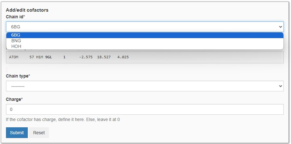
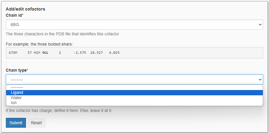
Here, we want to run the MD simulation in the presence of 6BG as it has been crystalized within the transporter channel. We start by heading to ‘Add a cofactor’ and we will be presented with the panel seen in Figure 4. Besides 6BG, we are also presented with BNG and HOH as these molecules are also present in 4gc0.pdb. Here we decide not to include the BNG (the nonyl beta-D-glucopyranoside molecules used for crystallization) and crystallized waters (HOH) molecules as they are not expected to have a major impact on the dynamics of the protein after membrane insertion. To add 6BG to our MD simulation we select it as our cofactor. Then we define the molecule type (see Figure 5) and charge. In this case, BNG is an organic ligand with a neutral charge. Finally, we press ‘Submit’ to add the cofactor to the MD simulation.

For additional notes on adding cofactors see ‘Additional notes on cofactors’.

Now we can press ‘Run MD’ and initialize the MD pipeline for our protein-ligand complex. Note, as we have not added BGN and HOH to our simulation, these will excluded from the MD simulations.

The MD simulation takes from 12h to 2 days, depending on the size of the protein. When the MD pipeline is finished, we can find the MD output by going to the ‘Projects’ tab > ‘Tutorial_4GC0’ > ‘1 associated Dynamic’ > ‘Dynamic for Pdb: PDB 4GC0_Tutorial’ > ‘Molecular Dynamics Results’. This downloads the file MD_output.tgz, containing the output files of the MD pipeline.

The MD pipeline starts with aligning the protein complex with the membrane. Firstly the protein is stripped from its cofactors in protein_stripped.pdb. The transmembrane membrane residues are identified using OPM after which they are aligned with the membrane (z-axis) in protein_aligned.pdb. Lastly, all added cofactors are reintroduced to the aligned protein resulting in homology.pdb. The structure is then ready for membrane embedding and MD simulation. Note that all these steps are automatically performed within the server.

In addition, the user is provided with a selection of files to allow for analysis of the protein embedding and MD simulation. hexagon.pdb contains the protein-membrane system after membrane insertion, which is used in the MD simulations. The final conformation of the protein-membrane system of the MD simulations is found in the 3D model file confout.gro. The MD simulation and specifications are provided within the trajectory- (.xtc format) and log files generated by GROMACS. The output includes a PyMOL script (.pml) that loads the trajectory. To investigate the protein characteristics during the MD simulations, RMSD and RMSF reports are provided. In addition, reports are generated for the total energy, pressure, temperature, and volume of the system All reports are found in the reports folder. Lastly, README.md contains all information required to thoroughly analyze the generated results, before putting the results to use in future projects.

Additional notes on cofactors

When adding cofactors, make sure all cofactors are present in the same uploaded PDB file. Multiple cofactors can be added to an MD simulation by repeating the process of adding a cofactor in ‘Add a cofactor’. In the following section, we will describe the different types of cofactors in more detail:

Ligands:

Any organic molecule present in the PDB file can be added by selecting the corresponding 3-letter code residue ID. This includes structures such as typical ligands, but also cholesterol, lipids, etc.. Multiple ligands can be added to the MD simulation, however each ligand must have a unique 3-letter code. The ITP and FF files with the corresponding OPLS parameters (needed for GROMACS to recognize the new molecules) are then automatically generated with LigParGen.

Note that hydrogens can only be automatically added if the total charge of the molecule is neutral (charge is 0). If your ligand has a formal charge, hydrogens must be explicit in the PDB file, as is required in the LigParGen web server. This is because proton addition on charged ligands is a complex task prone to bugs, thus outside of the scope of this pipeline.

Waters:

Crystalized waters can be added in bulk as a cofactor by selecting their common residue ID. All water molecules must have the hydrogens explicitly defined. Note that additional waters are added to the simulation when embedding the protein complex.

Ions:

Crystalized ions can be added in bulk as a cofactor by selecting their common residue ID. The residue IDs must use the mapping as described in Table 1. Note that additional ions are added to the simulation to neutralize the formal charge of the system. When the formal charge of the full system is positive, Cl- ions are added to neutralize the system. Alternatively, Na+ ions are added to neutralize systems with a negative formal charge.

Table 1. Mapping of ions to their corresponding residue IDs (ResID).

Ion	Br	Ca	Cl	Cs	F	I	K	Li	Mg	Na	Rb
ResID	BR	CA	CL CL- CHL	CS	F	I	K	LI	MG	NA NA+ SOD	RB